Scaling Stellar P-mode pulsations/oscillations
Or, an example of what my research can look like, and solving a minor problem to make simulations more realistic.
Stellar Pulsations
Stars are not just serene spheres sitting in the sky. For that matter, they’re not just spinning spheres with limb darkening (despite my implementation of Beatty and Gaudi 2015). They wobble and oscillate, with all sorts of acoustic waves bouncing through their interiors.
The P-mode Specifically
This is a “pressure” mode, and is the most important one in (more or less) sun-like stars. It’s a huge hassle for us in the RV community (because it adds a spurious signal), and so we want to remove it. The simple version is to observe the star for a timescale that’s comparable to the length of the oscillation, so it averages out. For the sun this is about 5 minutes, though it varies with stellar mass, radius, etc. Also, if you get it wrong, you get reduced RV precision.
In my (admittedly rather brief) initial search of the literature12345, it looked like the vast majority of the work is in characterization details. While useful for modeling the stellar interior, those details are unrelated to what I want (removing the “noise”). However, the typical timescale for the p-mode appears to more or less match up with the dynamical timescale:
\[τ_{dyn} = \sqrt{\frac{R^3}{GM}} = \sqrt{\frac{1}{G\rho}}\](Some older works apparently would divide the typical pulsation period by the dynamical timescale to show details in trends)
So I went with that. The p-mode compensation sets a minimum time (in seconds) of:
\[τ_{pmode} = 300 \sqrt{\frac{R^3}{M}}\]Where R and M are in solar units.
Immedately after running simulations with this, I found that some sources67 took a more sophisticated approach, using effective temperature and surface gravity:
\[ν_{max} = 3100 \ μHz \ \left(\frac{g}{g_{☉}}\right)^1 \ \left(\frac{T_{eff}}{T_{eff,☉}}\right)^{-0.5}\]Where the effective temperature is in kelvins and the surface gravity is in cm/s. However, normally surface gravity is given in \(log_{10}(cm/s)\), so I started with that.
My adopted values for solar surface gravity and effective temperature are: \(T_{eff,☉} = 5778 \ K\) and \(log(g_{☉}) = 4.438067627303176\)
Since my code works with a period instead of a frequency, I took one over this. (As an aside, one needs to be careful if using astropy’s units here, and tell it to explicitly convert to Hz and/or seconds.)
 A comparison of our two models, making the assumption that values scale such that (R,T as functions of M)
Realistic Stars
Using the HWO target list (at least as of 2023-07-26) from the NASA Exoplanet archive, this gives relative distributions of mass, radius, and dynamical times of:
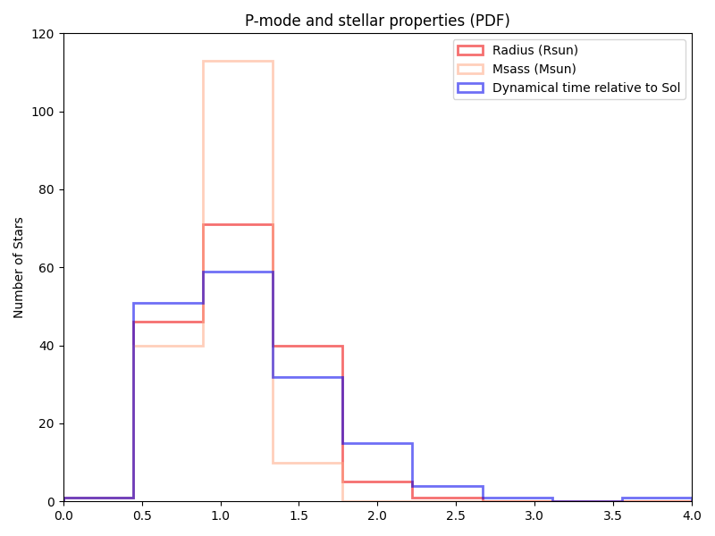
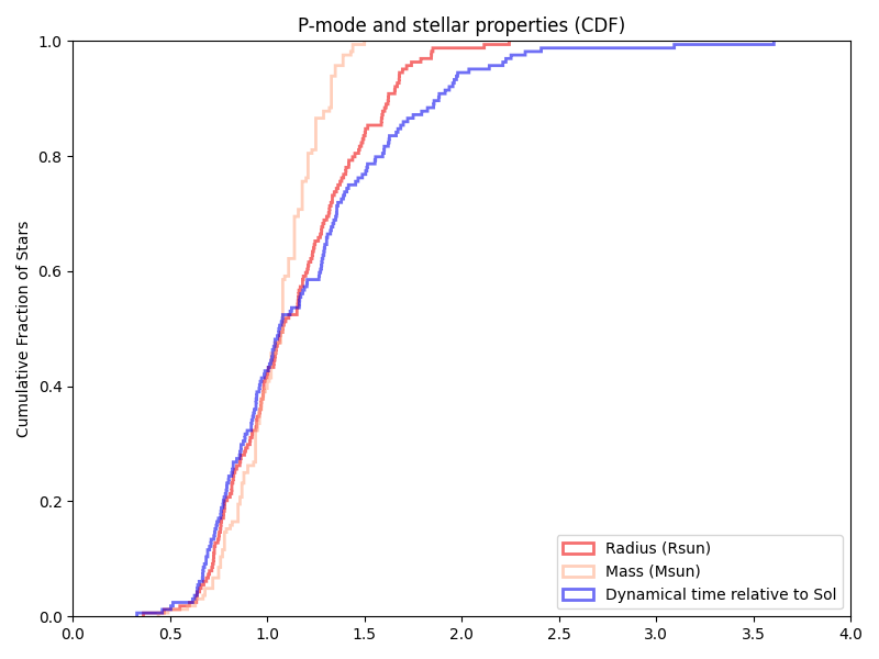
For comparison, the ‘old’ (HabEx at the time) target list that I assembled in the late 2010s (and we’ve more or less deprecated) is:
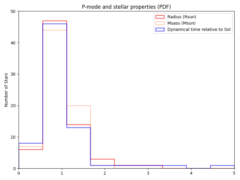
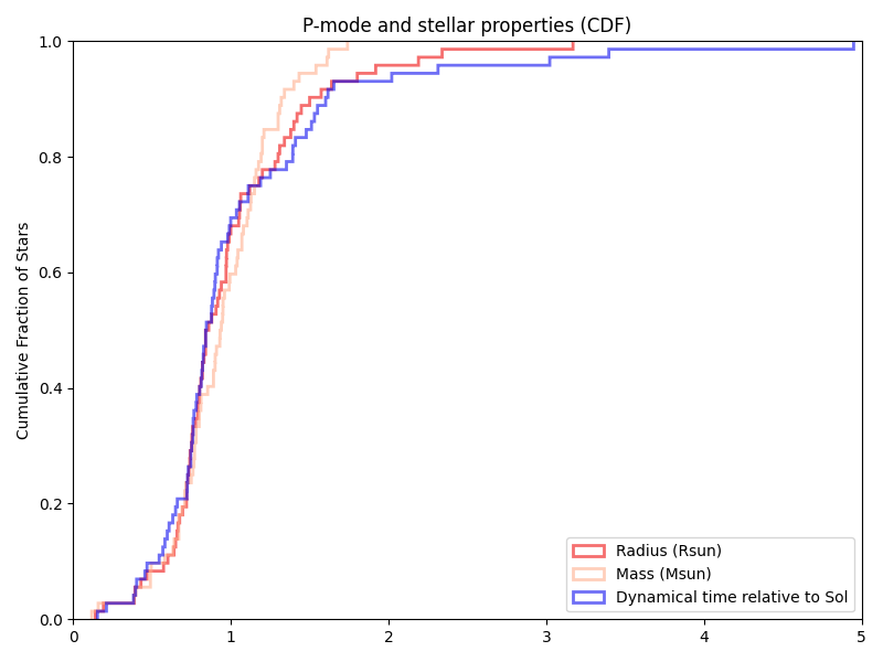
And the previous paper/technical report would have:
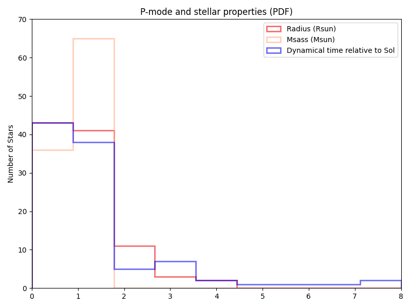
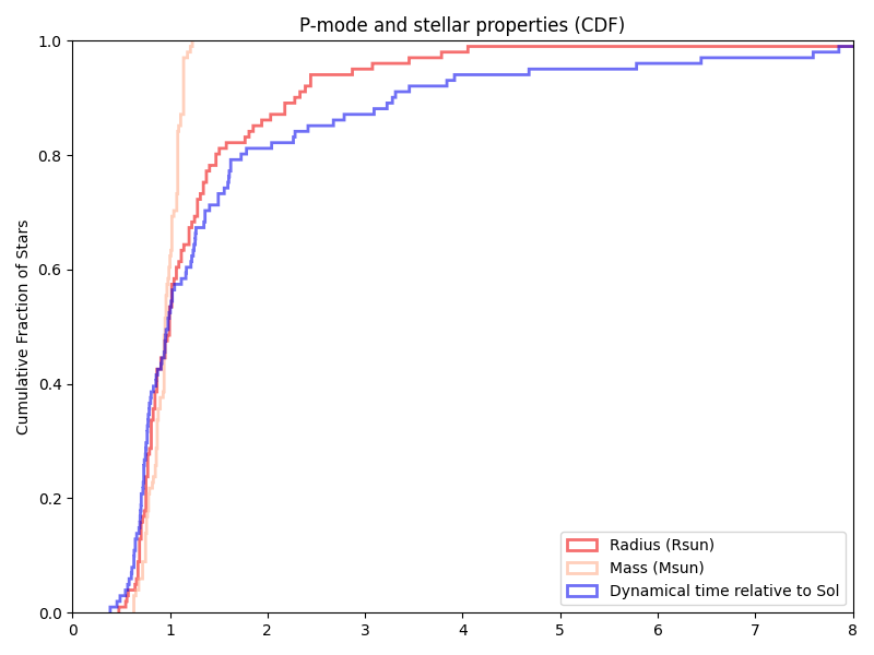
(though we only ran fixed 5 minute and 10 minute minimums there)
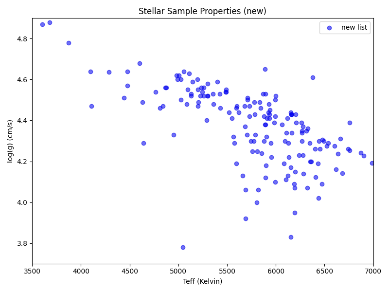
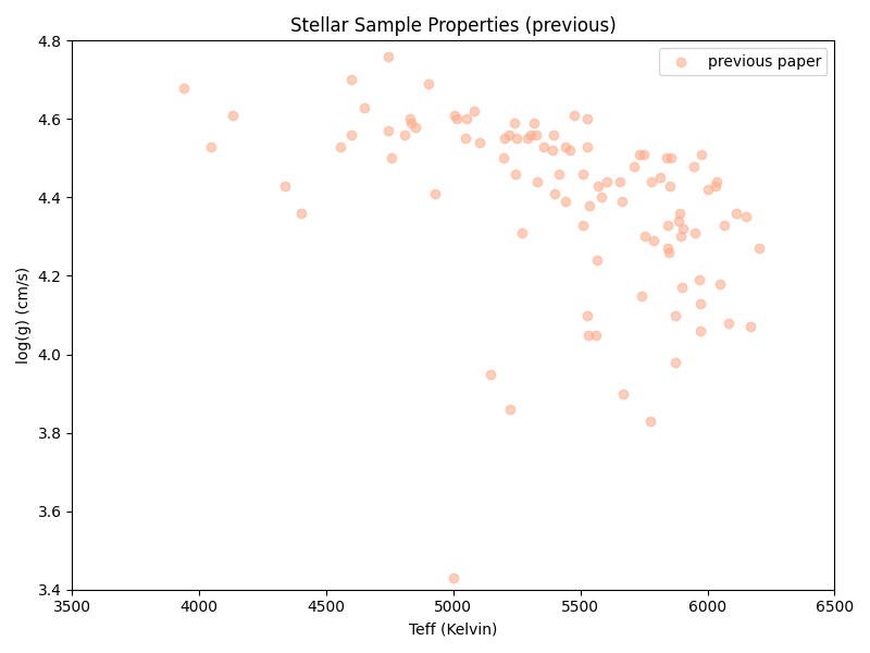
As for the stars themselves, the lists vary in size and there’s some overlap:
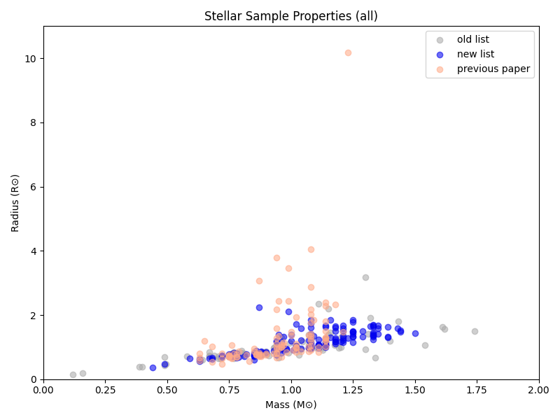
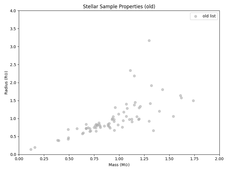
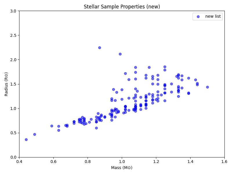
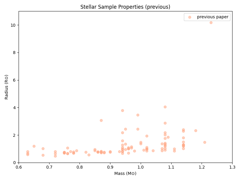
The target lists with other method
The actual stellar properties show up a bit differently, but you can still see similar overall patterns (if possibly flipped around, depending on axis choice. This is also part of why we sometimes have ‘backward’ axes in astronomy.)
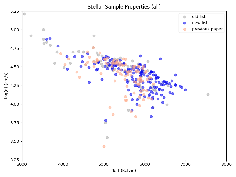
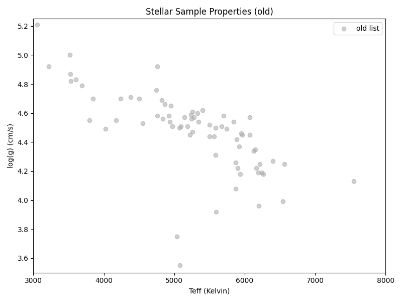
My first attempt (once units were fixed) at the actual scaling ended up with slightly odd results (from using the log instead of the actual surface gravity). While the baseline time is a bit different here (~322 seconds instead of 300), it’s multiplied by… almost 1:
In our new target list:
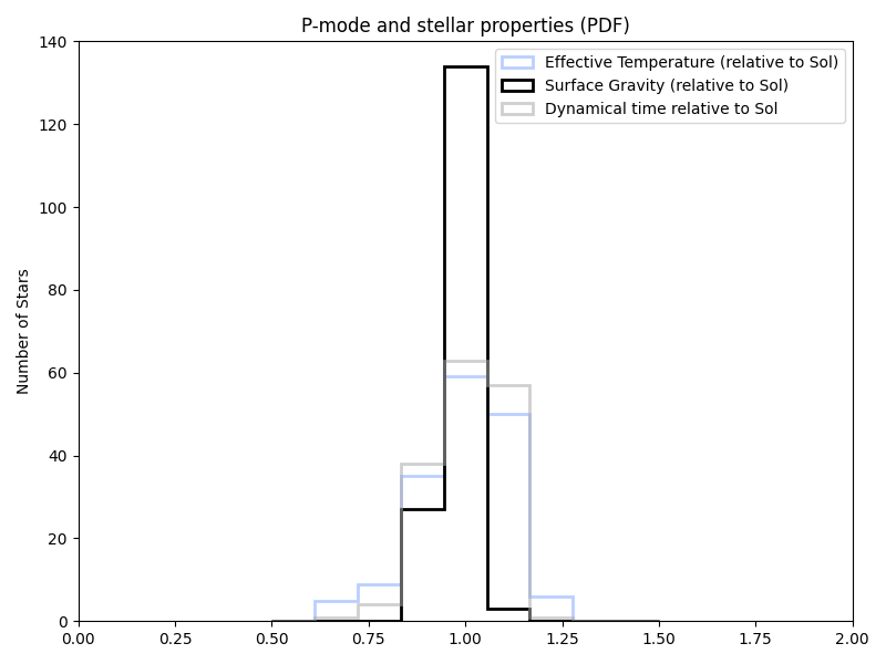
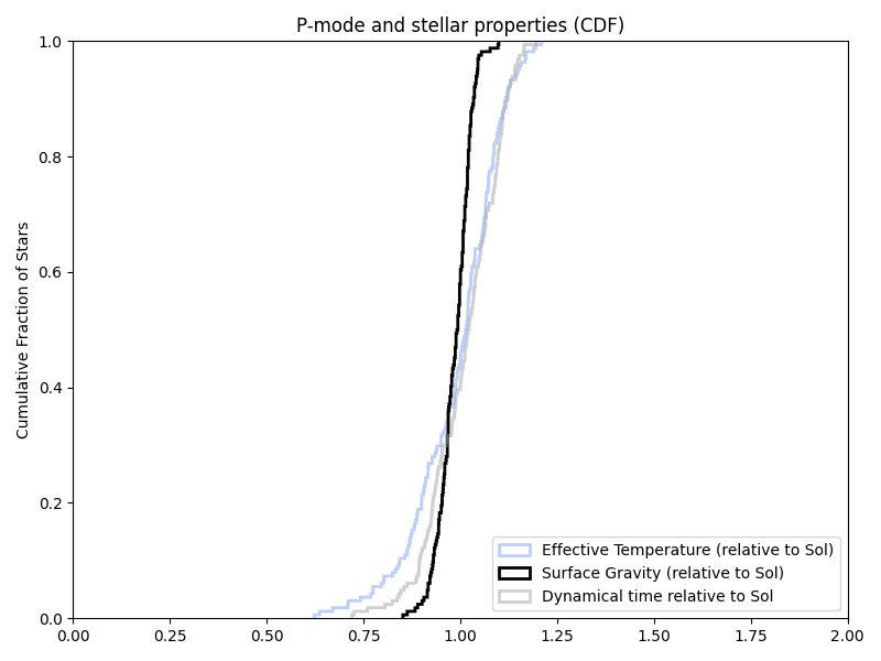
In the old target list:
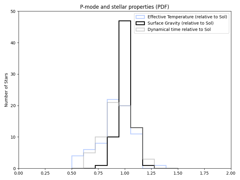
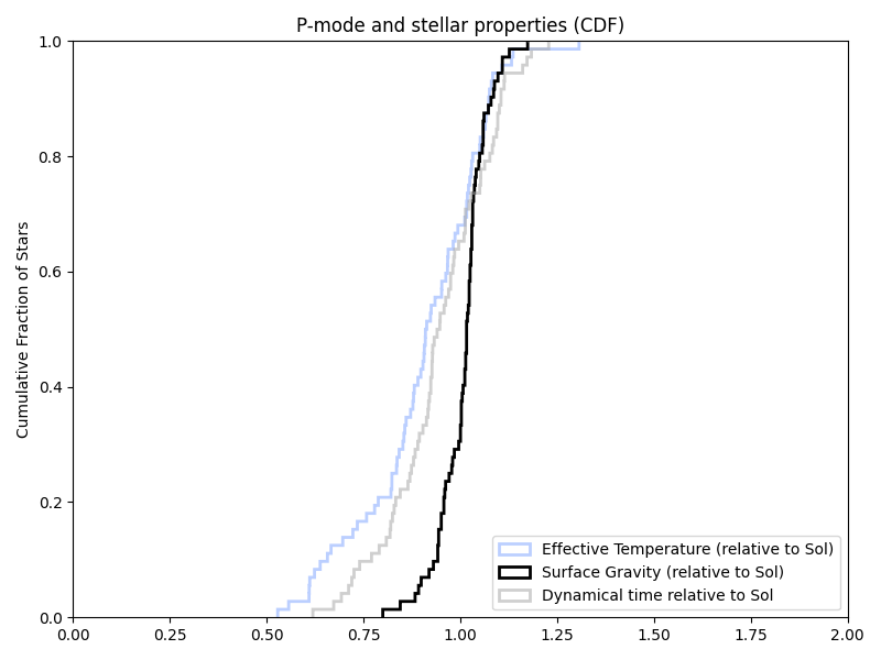
And in the previous paper’s target list:
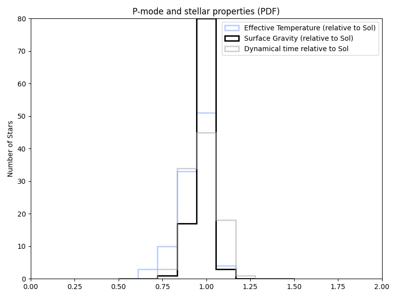
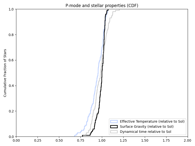
But all of this was assuming log(g). And the papers just listed g. So trying that (in new/old/previous target list order again):
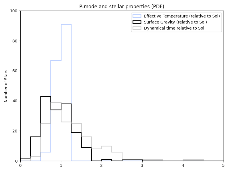
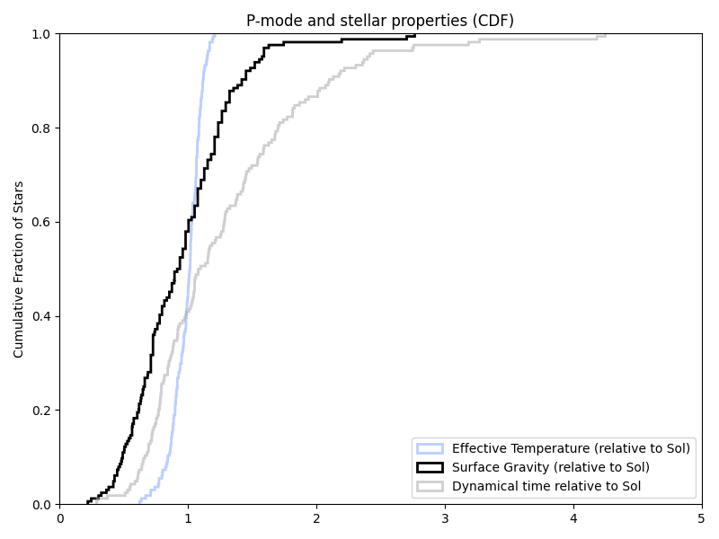
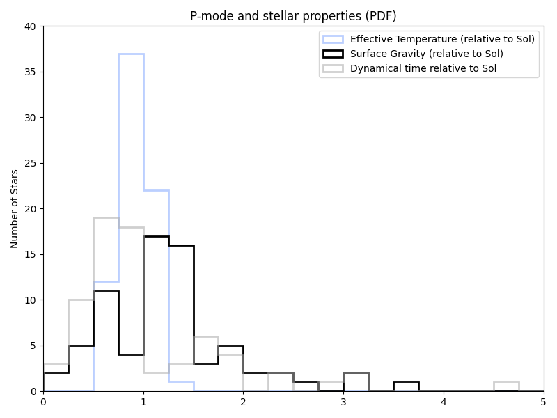
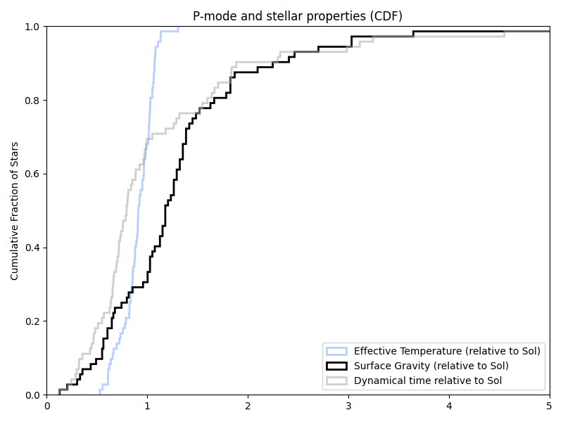
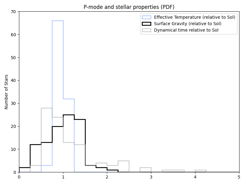
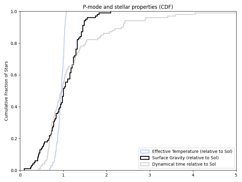
That certainly looks closer.
Actual Exposure Times
The details of the model are in my previous work (and Beatty 2015), but we do an estimate of stellar RV information based off model spectra that are scaled based on the star’s effective temperature, surface gravity, metallicity, macroturbulence (if available), and rotational velocity. All of which can have a rather larger effect than this bit of noise, depending on the telescope, instrument, star, and desired precision. But we can control for those with what amounts to a grid of simulations and/or choosing nominal instruments.
Exposure times with the HWO target list
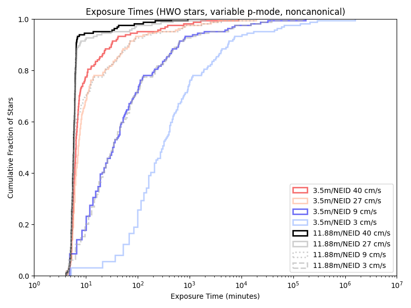
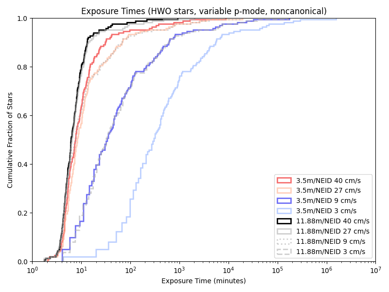
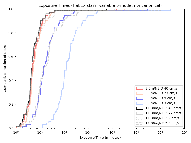
While we only have a few telescope/instrument/sensitivty combinations that are “canonical” (directly based on some actual instruments and probably extrapolations), simulations of combinations of all of them are computationally quite cheap. Looking at the CDFs (Cumulative Distribution FUnctions) of their exposure times. Using a visible light spectrograph nominally modeled on NEID:
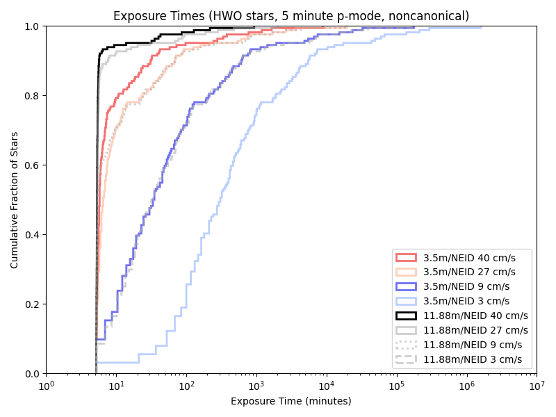

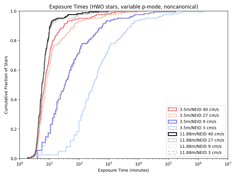
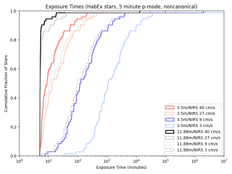
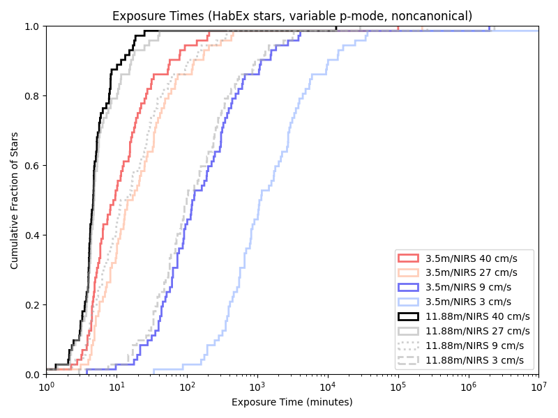
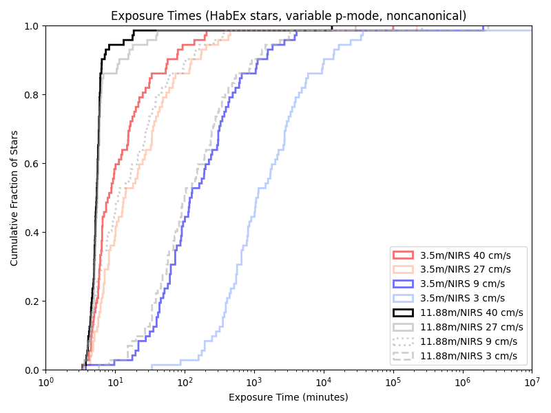
And on a near-IR spectrograph nominally modeled on iLocator:
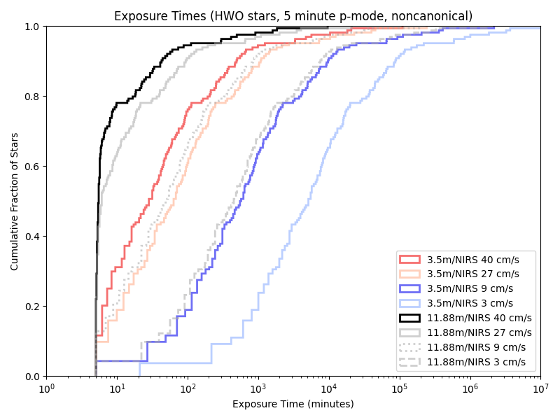

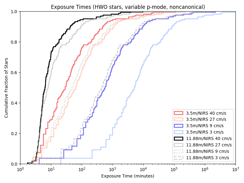
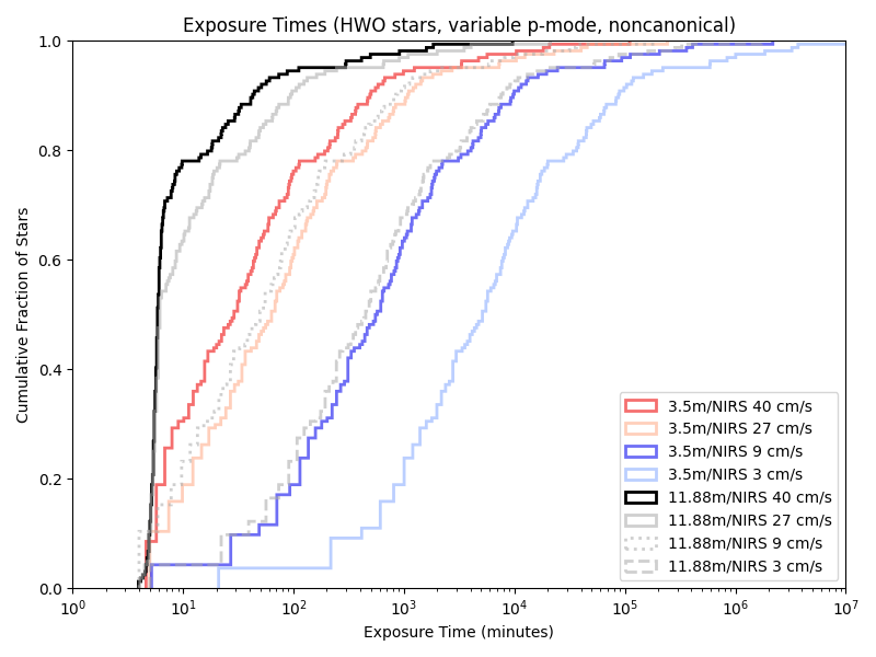
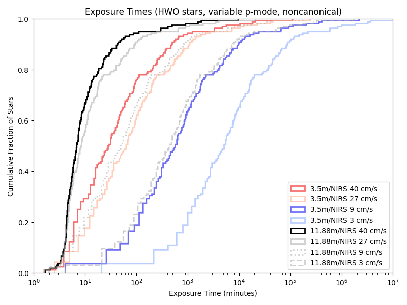
(While I’m using a 3.5 m telescope based off of the WIYN and an 11.88 m telescope that’s the combined LBT’s mirrors, there are also simulations for a single mirror “half-LBT”, with an 8.4 m aperture. But these graphs are already quite cluttered…)
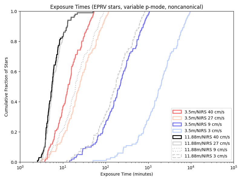
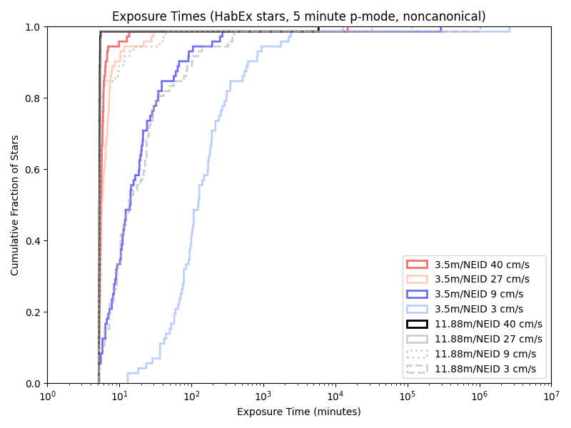
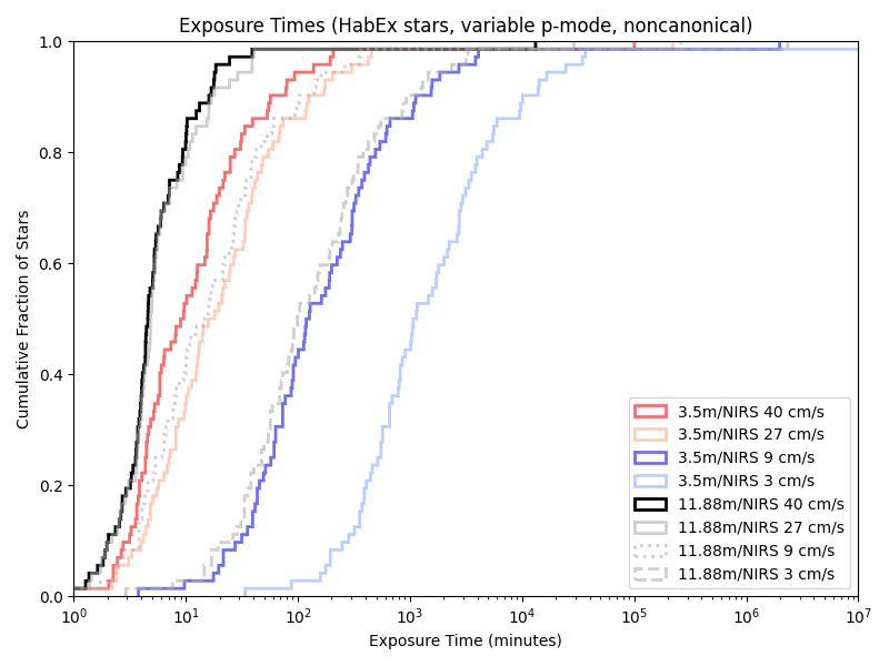
Given our previous 5/10 minute floors, a variable length minimum observation time rarely has an effect. Indeed, we’re only obseving short enough for it to matter with the combination of a large telescope and little care about photon noise!
Exposure times with the old/unsued (‘EPRV’) target list:
With the Neid analogue:
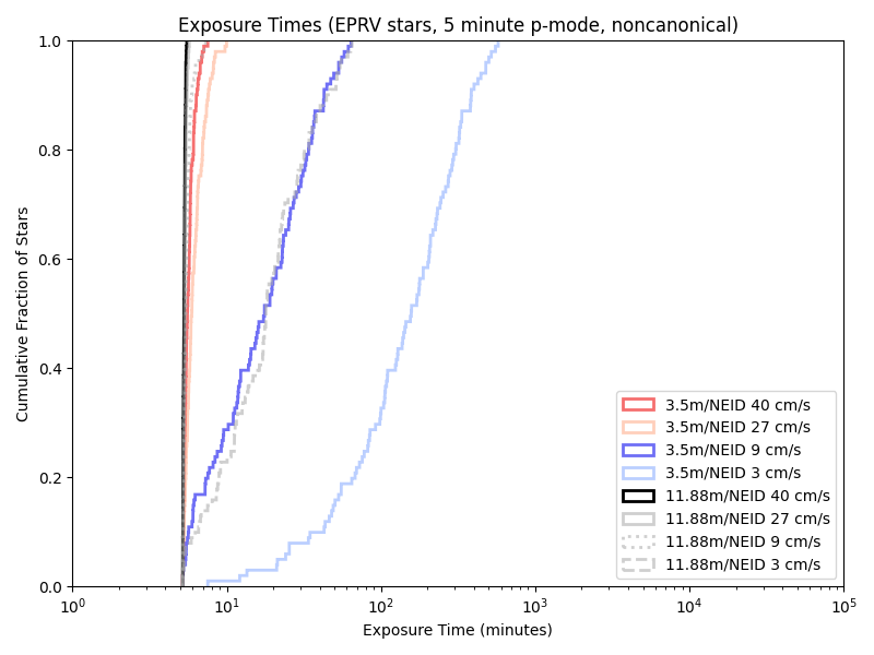

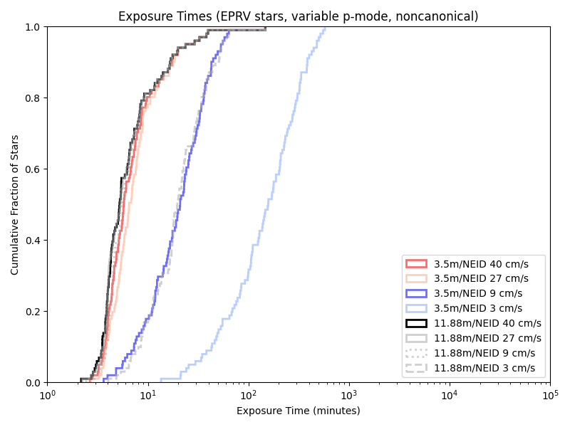
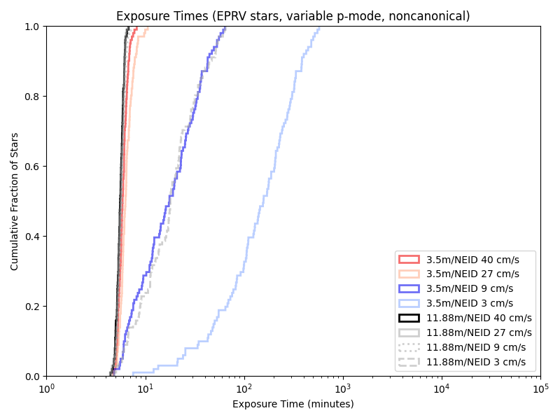
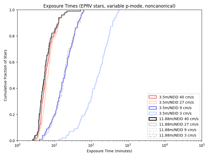
And the iLocator analogue:
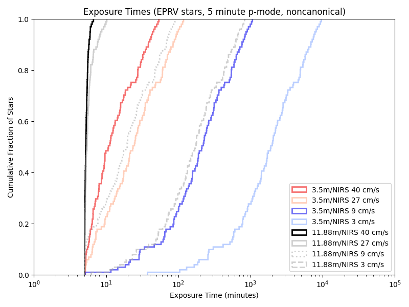

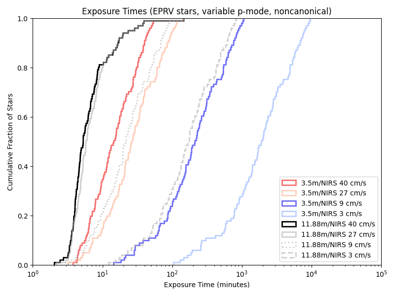

Exposure times with the previous paper (‘HabEx’) target list:
Neid:

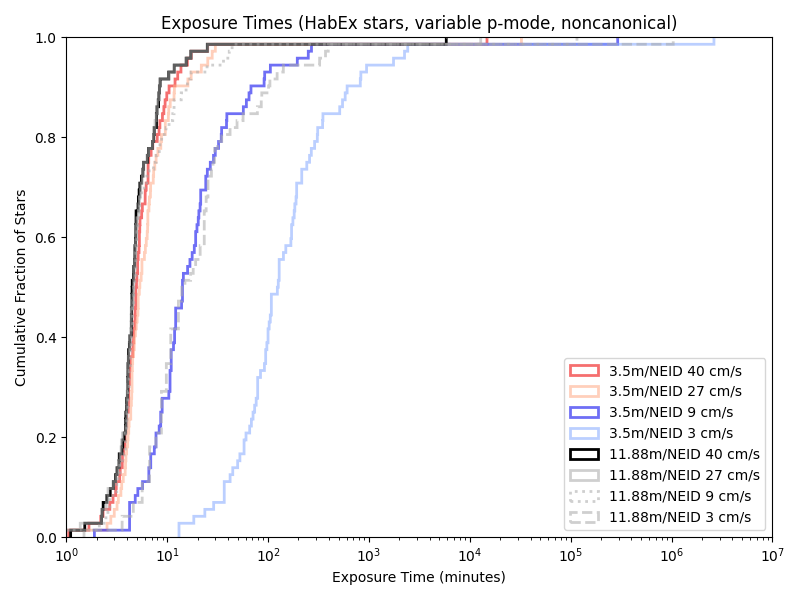
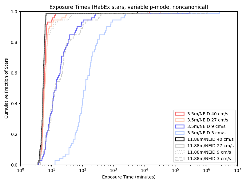
iLocator:

Conclusions
Actual details in terms of observations/precision, etc will be discussed in the paper (in prep). That said, perhaps this can make a case that we can finally kill p-mode oscillations as a noise source once and for all. Which “just” leaves things like granulation, spots/plages (and the associated magnetic activity cycles), flares, etc. (Which admittedly can have larger effects than what I’m mitigating here)
And, uh, I’m still mostly ignoring Earth’s atmosphere here. (Just general absorption with no microtellurics)
Once the paper is up, I’ll also want to put up these target lists. Stay tuned for more…